CDNF Part II: Take the namedtuples bowling

27 minute read

Reducing from Normal Form

The basics of reducing is that you need two terms like ABC and ABC’. This can be reduced to AB(C + C’). In Logic (C + C’) evaluates to 1–so you have AB(1) which is AB. Essentially the C and C’ cancel each other so you go from 2 terms, ABC and ABC’, to one term AB.

The general rules are:

Individual inputs must have a 1 to 1 match for inputs/letters. So ABC and ABD fail on this front.
Of the inputs only one can differ in its primed vs. unprimed form. So ABC and AB’C’ cannot be reduced. Extracting (C + C’) in this case leaves us with AB + AB’–which simply goes against the rules.
Finally, when performing reductions, terms of any generation can be used multiple times to come up with new terms.

I hope to make a lot of this clearer shortly, but for starters it is important to note that each generation will have the same number of inputs as all other items in the generation. For the bowling example the 1st generation will all have 4 inputs (and will also have the same set of inputs A, B, C, and D). 2nd generation will have 3 inputs–however, because of reduction, the set of inputs will not necessarily match. You could have terms with ABC and other terms with ACD. The 3rd generation will have 2 inputs in each term.

Situation 1 as an Example

So for Situation 1 we have the following terms in the 1st generation:

                ones    Ancestors
  ABCD       4       1
  ABCD'      3       2
  ABC'D      3       3
  ABC'D'     2       4
  AB'CD      3       5
  AB'CD'     2       6
  AB'C'D     2       7

Term 1 (ABCD) can be “minimized” with 3 other terms; 2, 3, and 5 (ABCD’, ABC’D, and AB’CD)–each of which differ from ABCD by having only 1 “primed” term. This results in 3 new 2nd generation terms–ABC, ABD, and ACD. ABC is derived from Term 1 (ABCD) and Term2 (ABCD’) to get ABC(D + D’) == ABC. ABD is T1 (ABCD) and T3 (ABC’D)–>ABD, etc.

Term 4 – Term2 and Term3 to get ABD’ and ABC’

Term 6 – Term2 and Term5 to get ACD’ and AB’C

Term 7 – Term3 and Term5 to get AC’D and AB’D

Generation 2 looks like:

            ones    Ancestors
 ABC     3       1, 2
 ABD     3       1, 3
ACD     3       1, 5
ABD'    2       4, 2
ABC'    2       4, 3
ACD'    2       6, 2
AB'C    2       6, 5
AC'D    2       7, 3
AB'D    2       7, 5

So for generation 2 we only have . . .

Term9 (ABD) and Term11 (ABD’) –> AB Ancestors(Term1, Term3, Term2, Term4)
Term10 (ACD) and Term13 (ACD’) –> AC Ancestors(Term2, Term6, Term1, Term5)
Term10 (ACD) and Term15 (AC’D) –> AD Ancestors(Term7, Term5, Term1, Term5)

Generation 3 ends up being:

            ones    Ancestors
AB      2       1, 3, 2, 4
AC      2       2, 6, 1, 5
AD      2       7, 5, 1, 5

For future reference things to note . . .

The ones column essentially helps us with Rule 2 above–terms can only differ by 1 item. ABC (111) has 3 ones, it can not be reduced with AB’C’ (100) as there is more than 1 different item (it has one 1). It can be compared with AB’C (101) as there are 2 ones. It could also be compared with ABD’ (11-0) but would fail based on rule 1.
The other item, may be the most important, is the ancestors. To form a complete reduction we need to have all the minterms from our original canonical form (generation 1) represented in our reduced terms. In this case generation 3; AB, AC, and AD; cover all 7 terms from the original canonical form. The ancestor lists for those 3 terms include 1, 2, 3, 4, 5, 6, and 7.
There is also no point in doing redundant minimizations. Term 8 (ABC) for example can be used to reduce with Term12 (ABC’) and Term14 (AB’C). But reducing T8 with T12 giving AB with 1, 2, 3, 4 as ancestors is the same as reducing T9 (ABD) with T11 (ABD’) with 1, 2, 3, 4 as ancestors. T8 with T14 similarly is the same as T10 and T13 to get AC with 1, 2, 5, 6 as ancestors.

Back to why this matters

It seems the most common case and use for reducing from a canonical form is with electronics/circuits. But as part of that whole “Turing Machine” thing it is actually something that occurs almost constantly in code–more often than not we are dealing with simpler cases and intuitively arrive at a minimized or close to minimized form.

Quine-McCluskey and Petrick’s Method (finally)

First some links:

In a nutshell–getting to a final minimized form involves using Quine-McClusky to reduce your terms from the canonical form. Once no more reduction is possible Petrick’s Method can be used to select a set of terms that will “cover” all the terms from the original canonical form.

Now for some code

So, we finally get to the namedtuple portion of our program. Throughout my implementation a list of namedtuples (term_list) is used for storing information on the terms and the reductions. The tuples definition is:

Term = namedtuple('Term', 'termset used ones source generation final')

Some of the named fields should be familiar from the example above. The major use for this is for the term_list variable that stores all of our generations and reductions. Within our “namedtuple” Term the fields are . . .

termset – these are actual python sets that will contain the inidividual inputs for a term. So ABC would be (“A”, “B”, “C”), ABD’ would be (“A”, “B”, “D’”).
used – this will be True or False. If a term is “used” that means it was used to create a term for a later generation and can be ignored in finding our final reduction.
ones – A simple count of the number of 1s or un-primed inputs. ABC would have this as 3, ABD’ would have it as 2. Ultimately we sort each generation by the “ones” column.
source – specifies which terms were used in creating this term. Generation 1 terms will have source set to themselves. Gen 2 would have items like (0, 3), Gen 3 would have (0, 3, 2, 4), etc.
generation – simply the generation of this item
final – by default it is “None”. After processing the items needed for our final reduction will have either “Required” or “Added” in this field.

The basic layout of the code/functions is . . .

quinemc implementation

quinemc()

To perform a reduction you’d simply call quinemc . . .

def quinemc(myitem, highorder_a=True, full_results=False):

myitem – can be an int, a string containing a canonical form, or a list containing terms from a canonical form. If you provide an int quinemc will call canonical(myitem) to get the canonical form. If you provide a string or list you’ll get an error if it is not a true canonical form (e.g. “ABC + ABD”).
highorder_a – like canonical() this determines whether A is the highorder bit or loworder bit. Default is A as highorder.
full_results – The default (False) simply returns the reduced form as a string. If set to True quinemc() returns 3 items
- A string of the reduced form
- The term_list list–a list containing all of the Term namedtuples
- For some reductions there will be multiple ways to create a final form. If this is the case the 3rd item will be a dictionary containing all of the possible completions.

Examples

quinemc(65024)
quinemc("ABCD + ABCD' + ABC'D + ABC'D' + AB'CD + AB'CD' + AB'C'D")
quinemc(["ABCD", "ABCD'", "ABC'D", "ABC'D'", "AB'CD", "AB'CD'", "AB'C'D"])
a, b, c = quinemc(65024, full_results=True)

All 4 are equivalent and give “AB + AC + AD” as a result.

quinemc() itself just validates that the input is either an int, string, or list. Then also validates that the input item is in fact a canonical form (lines 11-14). From there it simply calls _minimize_() where the real processing takes place. In case you are wondering the cdnf variable is just a list of the terms like . . .

['ABCD', "ABCD'", "ABC'D", "ABC'D'", "AB'CD", "AB'CD'", "AB'C'D"]

_minimize_()

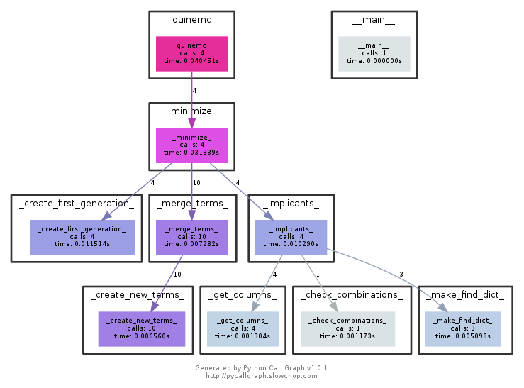
_minimize_() is essentially the driver function. It simply calls 3 other functions. The first two (in order), _create_first_generation_ and _merge_terms_ are the Quine-McCluskey portion. The last, _implicants_, is the Petrick method portion that finds our final result(s).

The final bit of code handles special cases. The first is for a zero input. The second is for cases like quinemc(15) or quinemc(255) where all the terms end up canceling out.

_create_first_generation_()

For our first step we are simply taking the terms from our canonical form and putting them into the term_list namedtuple. For situation 1, quinemc(65024), we get a 1st gen term_list of . . .

Term(termset={"C'", 'A', 'B', "D'"}, used=False, ones=2, source=[0], generation=1, final=None)  
Term(termset={'A', 'C', "D'", "B'"}, used=False, ones=2, source=[1], generation=1, final=None)  
Term(termset={"C'", 'A', "B'", 'D'}, used=False, ones=2, source=[2], generation=1, final=None)  
Term(termset={'A', 'C', 'B', "D'"}, used=False, ones=3, source=[3], generation=1, final=None)  
Term(termset={"C'", 'A', 'B', 'D'}, used=False, ones=3, source=[4], generation=1, final=None)  
Term(termset={'A', 'C', "B'", 'D'}, used=False, ones=3, source=[5], generation=1, final=None)  
Term(termset={'A', 'C', 'B', 'D'}, used=False, ones=4, source=[6], generation=1, final=None)  

This is simply taking the 7 terms from our canonical form and putting them into the “Term” namedtuple data structure. The first bit of code converts our terms to python sets (line 3). Line 6 exists only to clean up duplicate terms if quinemc was called with a string or list. Lines 8/9 actually creates our Term namedtuple. We then sort it by the number of “ones” at line 10 and then update our namedtuple with each items index at lines 11 & 12. (_replace is something from the namedtuple item–essentially a short cut for updating an immutable object. As the name implies it isn’t “updating” the immutable tuple but is replacing it with a copy of the original and a single value changed.)

As far as our “Term” namedtuple goes–_merge_terms_ will use python set functions so “termset” puts our terms into “sets”. The “used” flag will also be used by merge_terms; ultimately only items that are still used=False will be potential terms for our final result. As noted before it only makes sense to compare terms where the number of “ones” differs by 1 so the whole list is sorted by how many “ones” are in a term.

For our first generation the “source” list is essentially a reference to the item itself. This simplifies things in merge_terms so that we do not need to use list indexes for our first gen items.

“generation” is another item used by _merge_terms_. Again, it only makes sense to compare/reduce items that exist in the same generation as the number of inputs needs to match. Each successive generation will reduce the number of items in the “termset” by one. So, as in this case, Generation 1 has 4 inputs; if we can reduce anything then all Generation 2 items will have 3 inputs; if Gen 2 items can be reduced all Generation 3 items will have 2 inputs; finally if possible Generation 4 would have termsets with a single input.

“final” is ultimately used by the _implicants_/Petrick’s method part of the code.

_merge_terms_ and _create_new_terms_

_merge_terms_ is pretty simple. It is called for each generation and it then tries to minimize that generation. When nothing can be minimized done becomes True.

_create_new_terms_ is where we perform our actual reductions. Taking terms like ABC and ABC’ to get AB. working_list is simply a stripped down version of our term_list variable containing only items for the current “generation”. Lines 21 and 22 do a nested loop over the items in working_list.

The “tricky” bit is the “sym_set” variable. Line 24 does a set comparison of our term_list.termset items and gets a “difference” set on them. So comparing ABC to ABC’ results in a “sym_set” of (C, C’). Line 26 then checks whether we have only 2 items in our “sym_set”–this would fail if we had AB’C’ and ABC. Then also checks that the inputs (e.g. C) match – list(sym_set)[0][0] == list(sym_set)[1][0]. If that all works out we then create a new merged term.

Lines 31 - 36 avoid doing duplicate sources for reductions.

After all of this work is done the used_dict dictionary is used to update our global term_list to mark all items that have been used in merges.

At this point our term_list looks like . . .

Term(termset={'B', 'A', "C'", "D'"}, used=True, ones=2, source=[0], generation=1, final=None)
Term(termset={"B'", 'C', 'A', "D'"}, used=True, ones=2, source=[1], generation=1, final=None)
Term(termset={"B'", 'A', "C'", 'D'}, used=True, ones=2, source=[2], generation=1, final=None)
Term(termset={'B', 'C', 'A', "D'"}, used=True, ones=3, source=[3], generation=1, final=None)
Term(termset={'B', 'A', "C'", 'D'}, used=True, ones=3, source=[4], generation=1, final=None)
Term(termset={"B'", 'C', 'A', 'D'}, used=True, ones=3, source=[5], generation=1, final=None)
Term(termset={'B', 'C', 'A', 'D'}, used=True, ones=4, source=[6], generation=1, final=None)
Term(termset={'B', 'A', "D'"}, used=True, ones=2, source=[0, 3], generation=2, final=None)
Term(termset={'B', 'A', "C'"}, used=True, ones=2, source=[0, 4], generation=2, final=None)
Term(termset={'C', 'A', "D'"}, used=True, ones=2, source=[1, 3], generation=2, final=None)
Term(termset={"B'", 'C', 'A'}, used=True, ones=2, source=[1, 5], generation=2, final=None)
Term(termset={'A', "C'", 'D'}, used=True, ones=2, source=[2, 4], generation=2, final=None)
Term(termset={"B'", 'A', 'D'}, used=True, ones=2, source=[2, 5], generation=2, final=None)
Term(termset={'B', 'C', 'A'}, used=True, ones=3, source=[3, 6], generation=2, final=None)
Term(termset={'B', 'A', 'D'}, used=True, ones=3, source=[4, 6], generation=2, final=None)
Term(termset={'C', 'A', 'D'}, used=True, ones=3, source=[5, 6], generation=2, final=None)
Term(termset={'B', 'A'}, used=False, ones=2, source=[0, 3, 4, 6], generation=3, final=None)
Term(termset={'C', 'A'}, used=False, ones=2, source=[1, 3, 5, 6], generation=3, final=None)
Term(termset={'A', 'D'}, used=False, ones=2, source=[2, 4, 5, 6], generation=3, final=None)

Major things to note–the generations I think are clearer here. The _merge_terms_ function has set “used” to true for everything in Gen 1 and Gen 2. Looking at Gen 2 you can see in the source column that all 7 items (0-6) have been used. Generation 3 points to an important part of the code in this regard. Line 32 of _create_new_terms_ prevents us from doing duplicate “merges”, but the preceding lines (28 and 29) mark the items we aren’t actually using as duplicates as far as “used” is concerned.

The for loop at lines 39 - 42 is the code that actually goes through and marks the individual terms as “used”. This ends the Quine-McCluskey portion of the reduction. For Petrick’s method we will only need to consider the Term items that have “used=False”.

If you look at the Simplifying with Quine-McCluskey Method section at Circuits and Petrick The table under “Now to find the prime implicants:” is essentially what we have accomplished. Each of the 3 columns represent a generation. Within a generation the terms are grouped by the number of 1s. And finally check marks have been added for each term that has been used in a reduction.

Petrick’s Method

From Situation 1 we have ended up with 3 terms that may be needed to form our final result.

Term(termset={'B', 'A'}, used=False, ones=2, source=[0, 3, 4, 6], generation=3, final=None) Term(termset={'C', 'A'}, used=False, ones=2, source=[1, 3, 5, 6], generation=3, final=None) Term(termset={'A', 'D'}, used=False, ones=2, source=[2, 4, 5, 6], generation=3, final=None)

On paper starting Petrick’s method would require putting this into a table form with 1 column for each term from our canonical form (generation 1) and a row for each term that hasn’t been used. The remainder of the grid is filled in using the “source” values for the terms–with the goal being to find a set of terms that “fills” all of the columns.

    0   1   2   3   4   5   6
---------------------------------
AB  x           x   x       x    
AC      x       x       x   x
AD          x       x   x   x

A “required” prime implicant can be found by finding columns that only contain 1 “x”–that essentially means that term is the only one that “covers” the corresponding term from the canonical form. In this case columns 0, 1, and 2 all have single x’s and they are each for one of our 3 terms.

The other consideration is that all terms from the canonical form must be covered. In this case this is met using the 3 “required” terms. (In fact any time when all of the “used=False” terms are required terms they would cover all of the canonical terms.)

Situation 2 is slightly more interesting. In that case the final reduction looks like . . .

Term(termset={'B', "D'", "C'", 'A'}, used=True, ones=2, source=[0], generation=1, final=None) Term(termset={"D'", "B'", 'C', 'A'}, used=True, ones=2, source=[1], generation=1, final=None) Term(termset={"C'", "B'", 'D', 'A'}, used=True, ones=2, source=[2], generation=1, final=None) Term(termset={'B', "C'", 'D', 'A'}, used=True, ones=3, source=[3], generation=1, final=None) Term(termset={"B'", 'C', 'D', 'A'}, used=True, ones=3, source=[4], generation=1, final=None) Term(termset={'B', "C'", 'A'}, used=False, ones=2, source=[0, 3], generation=2, final='None') Term(termset={'A', "B'", 'C'}, used=False, ones=2, source=[1, 4], generation=2, final='None') Term(termset={"C'", 'D', 'A'}, used=False, ones=2, source=[2, 3], generation=2, final=None) Term(termset={"B'", 'D', 'A'}, used=False, ones=2, source=[2, 4], generation=2, final='None')

In this case the canonical form only has 5 terms and the reduction is complete with generation 2–and all of the generation 2 items have “used=False”. In this case our table looks like . . .

        0   1   2   3   4
--------------------------
ABC'    x           x
AB'C        x           x
AC'D            x   x
AB'D            x       x

In this case only the 1st 2 terms are required (ABC’ and AB’C) because columns 0 and 1 are the only ones with a single X. But we still need to make sure all of the terms from the original canonical form are covered. ABC’ covers 0 and 3, AB’C cover 1 and 4. So the only “uncovered” item is term 2–both AC’D and AB’D will take care of column 2. Since they are both the same length we could use either one so . . .

ABC’ + AB’C + AC’D and ABC’ + AB’C + AB’D

are equivalent. And logically this makes sense if you consider the Situation 2 story where Bob and Clara won’t bowl together.

Ultimately, for the code purposes, none of our 4 situations actually exercise all of the code (they really are pretty simple situations). For that I’ll be using 2046 (‘0b11111111110’). canonical(2046) and quinemc(2046) give us . . .

“AB’CD’ + AB’C’D + AB’C’D’ + A’BCD + A’BCD’ + A’BC’D + A’BC’D’ + A’B’CD + A’B’CD’ + A’B’C’D” and “AB’D’ + B’C’D + A’B + A’C”

I really have no idea what Alan, Bob, Clara and Declan are doing here, but again note the canonical form starts with 10 terms corresponding to the number of 1’s in the binary representation. After reduction we end up with . . .

Term(termset={"D'", "C'", "B'", 'A'}, used=True, ones=1, source=[0], generation=1, final=None) Term(termset={'B', "C'", "A'", "D'"}, used=True, ones=1, source=[1], generation=1, final=None) Term(termset={"D'", "B'", "A'", 'C'}, used=True, ones=1, source=[2], generation=1, final=None) Term(termset={"C'", "B'", 'D', "A'"}, used=True, ones=1, source=[3], generation=1, final=None) Term(termset={"D'", "B'", 'C', 'A'}, used=True, ones=2, source=[4], generation=1, final=None) Term(termset={"C'", "B'", 'D', 'A'}, used=True, ones=2, source=[5], generation=1, final=None) Term(termset={'B', "D'", "A'", 'C'}, used=True, ones=2, source=[6], generation=1, final=None) Term(termset={'B', "C'", 'D', "A'"}, used=True, ones=2, source=[7], generation=1, final=None) Term(termset={"B'", 'D', "A'", 'C'}, used=True, ones=2, source=[8], generation=1, final=None) Term(termset={'B', 'D', "A'", 'C'}, used=True, ones=3, source=[9], generation=1, final=None) **Term(termset={"D'", "B'", 'A'}, used=False, ones=1, source=[0, 4], generation=2, final='None') **Term(termset={"C'", "B'", 'A'}, used=False, ones=1, source=[0, 5], generation=2, final=None) Term(termset={'B', "D'", "A'"}, used=True, ones=1, source=[1, 6], generation=2, final=None) Term(termset={'B', "C'", "A'"}, used=True, ones=1, source=[1, 7], generation=2, final=None) **Term(termset={"D'", "B'", 'C'}, used=False, ones=1, source=[2, 4], generation=2, final=None) Term(termset={"D'", "A'", 'C'}, used=True, ones=1, source=[2, 6], generation=2, final=None) Term(termset={"B'", "A'", 'C'}, used=True, ones=1, source=[2, 8], generation=2, final=None) **Term(termset={"C'", 'D', "B'"}, used=False, ones=1, source=[3, 5], generation=2, final='None') Term(termset={"C'", 'D', "A'"}, used=True, ones=1, source=[3, 7], generation=2, final=None) Term(termset={"B'", 'D', "A'"}, used=True, ones=1, source=[3, 8], generation=2, final=None) Term(termset={'B', "A'", 'C'}, used=True, ones=2, source=[6, 9], generation=2, final=None) Term(termset={'B', 'D', "A'"}, used=True, ones=2, source=[7, 9], generation=2, final=None) Term(termset={'D', "A'", 'C'}, used=True, ones=2, source=[8, 9], generation=2, final=None) **Term(termset={'B', "A'"}, used=False, ones=1, source=[1, 6, 7, 9], generation=3, final='None') **Term(termset={"A'", 'C'}, used=False, ones=1, source=[2, 6, 8, 9], generation=3, final='None') **Term(termset={'D', "A'"}, used=False, ones=1, source=[3, 7, 8, 9], generation=3, final=None)

I’ve added “**” in front of the unused terms just to highlight the sporadic locations of unused terms. The short list of only items where “used=False” is . . .

Term(termset={"D'", "B'", 'A'}, used=False, ones=1, source=[0, 4], generation=2, final='None') Term(termset={"C'", "B'", 'A'}, used=False, ones=1, source=[0, 5], generation=2, final=None) Term(termset={"D'", "B'", 'C'}, used=False, ones=1, source=[2, 4], generation=2, final=None) Term(termset={"C'", 'D', "B'"}, used=False, ones=1, source=[3, 5], generation=2, final='None') Term(termset={'B', "A'"}, used=False, ones=1, source=[1, 6, 7, 9], generation=3, final='None') Term(termset={"A'", 'C'}, used=False, ones=1, source=[2, 6, 8, 9], generation=3, final='None') Term(termset={'D', "A'"}, used=False, ones=1, source=[3, 7, 8, 9], generation=3, final=None)

From this our table would look like . . .

        0   1   2   3   4   5   6   7   8   9
---------------------------------------------
AB'D'   x               x    
AB'C'   x                   x    
B'CD'           x       x    
B'C'D               x       x
A'B         x                   x   x       x
A'C             x               x       x   x
A'D                 x               x   x   x

In this case the only required term is A’B as column 1 is the only one with a single x. It is probably obvious that shorter terms from later generations have more sources/ancestors–so they will often take care of larger groups. Anyway, removing A’B and all of the columns it covers (1, 6, 7, 9) gives us . . .

        0   2   3   4   5   8
------------------------------
AB'D'   x           x    
AB'C'   x               x    
B'CD'       x       x    
B'C'D           x       x
A'C         x               x
A'D             x           x

From this table it should be obvious that you’ll need either AB’D’ or AB’C’ to cover column 0, and you’ll also need one of A’C or A’D to cover column 8. I personally think doing this by hand is a pain–but ultimately you end up with 2 equivalent alternatives

“AB’D’ + B’C’D + A’B + A’C”
“AB’C’ + B’CD’ + A’B + A’D”

Petrick’s Method and the _implicants_ code

Going back to the call graph _implicants_() uses 3 functions–_get_columns_(), _make_find_dict_(), and _check_combinations_().

Our first order of business in _implicants_ is to make one large list containing all of the “source=[]” items from our terms where used=False. (Lines 5 and 6) This list will contain duplicates as it is used to find the required sources on Line 8 where we look for sources that appear once. For quinemc(2046) this list looks like . . .

[0, 4, 0, 5, 2, 4, 3, 5, 1, 6, 7, 9, 2, 6, 8, 9, 3, 7, 8, 9]

So, we have “0, 4” for AB’D’, then “0, 5” for AB’C’, etc. The only source that appears only once is 1–so our required list ends up looking like [1].

With that information in hand we now move onto _keep_columns_(). At this point the code starts to use some set operations and there are more of those to come. The major function of this code is to A) find and mark “required” terms and B) create two python sets: 1) the sources from our required items and 2) one containing the sources for the rest or the terms.

The for loop on lines 5 - 10 handles this. We “enumerate()” over the term_list where used=False–enumerate is important because we will need the index in term_list to update the “required” items.

Line 6 – we perform set intersection of required and the current terms sources. An intersection will return any values that are in both sets. The items in “required” will only be in one of our term’s source lists; however a term could potentially cover more than one required item which is why line 6 used >= 1.
Lines 7 & 8 – if our current term is required we update term_list and set final=”Required”. We also add the sources for the required term to our ignore list–it is a list at this point.
Line 10 – if our current term isn’t required we add its sources to a “keep” list
Line 12 – finally we generate a list of everything that is in “keep” but not in “ignore” by treating them as sets and using the set difference operator.

So for quinemc(2046) after the for loop “keep” contains [0, 4, 0, 5, 2, 4, 3, 5, 2, 6, 8, 9, 3, 7, 8, 9]. Ignore contains [1, 6, 7, 9]. And the final result after performing a set difference on the 2 is [0, 2, 3, 4, 5, 8]. Which is the same as the table above–we’ve removed the source items for the A’B term and marked that term as “Required”.

For something like our Situation 1 (quinemc(65024)) “keep” will end up empty as the 3 terms cover all terms from the canonical expression. Back in _implicants_ this situation is covered on line 11 where we set “finished” to True so we can skip the next bits of processing.

Our next little bit of code in _implicants_ is lines 13 through 19 which essentially checks to see if a single term will cover the remaining columns. It first, however, makes a detour to create “find_dict” by calling _make_find_dict_

_make_find_dict_

At this point in _implicants_ we have “keep_columns” which tells us which columns we still need to include in our final result. However, in our big “term_list” list each term still contains the columns we want to ignore in their “source” items. _make_find_dict_ addresses this by creating a dictionary containing a terms index from “term_list” along with a new namedtuple containing that term_list item’s sources with columns we want to ignore removed. This simplifies later set operations and our new namedtuple also includes a “length” item as it is possible to find many different reductions but some can be longer than others. It also covers the situation where an item in “term_list” can be completely ignored because the ancestors/sources it covers are already covered by a required item.

To illustrate what is going on–for quinemc(2046) our current term_list of “used=False” items (with term_list indexes) is . . .

Term(termset={"B'", 'A', "D'"}, used=False, ones=1, source=[0, 4], generation=2, final='None')
Term(termset={"B'", "C'", 'A'}, used=False, ones=1, source=[0, 5], generation=2, final=None)
Term(termset={"B'", 'C', "D'"}, used=False, ones=1, source=[2, 4], eneration=2, final=None)
Term(termset={"B'", "C'", 'D'}, used=False, ones=1, source=[3, 5], generation=2, final='None')
Term(termset={"A'", 'B'}, used=False, ones=1, source=[1, 6, 7, 9], generation=3, final='Required')
Term(termset={'C', "A'"}, used=False, ones=1, source=[2, 6, 8, 9], generation=3, final='None')
Term(termset={'D', "A'"}, used=False, ones=1, source=[3, 7, 8, 9], generation=3, final=None)

Note 23 (A’B) is marked as required and so we want to ignore [1, 6, 7, 9]. When _make_find_dict_() is finished we end up with a find_dict that looks like . ..

search_tuple(sourceSet={0, 4}, length=3)
search_tuple(sourceSet={0, 5}, length=3)
search_tuple(sourceSet={2, 4}, length=3)
search_tuple(sourceSet={3, 5}, length=3)
search_tuple(sourceSet={8, 2}, length=2)
search_tuple(sourceSet={8, 3}, length=2)

For 10, 11, 14, and 17 nothing changes; for 24 and 25 [6, 9] and [7, 9] (respectively) have been removed. And length is the length of each item’s term.

Final Step – _check_combinations_

After _make_find_dict_() we head back into _implicants_() and back into lines 13-19 where we are checking to see if a single term will complete our minimized form.

    if not finished:
        find_dict = _make_find_dict_(term_list, keep_columns)
        for idx, val in find_dict.items():
            if set(keep_columns) == val.sourceSet:
                term_list[idx] = term_list[idx]._replace(final="Added")
                finished = True
                break

At this point we have the new “find_dict” dictionary and “keep_columns” which contains the columns/canonical terms we still need to cover. The for loop at 15-19 (for idx, val ...) simply loops through our newly created “find_dict” and checks whether any of the “sourceSet” items there are an exact match for “keep_columns”. If any one item does cover all the needed columns then we are done–we simply update “term_list” at the index taken from find_dict’s key and set that term_list item’s final attribute to “added”.

So ultimately the final attribute within term_list will have one of 3 values . . .

None – The default. The term is not used in our final minimized form
Required – Denotes prime implicant set in _get_columns_(). Again, these are terms that are the only ones that cover one or more of our original canonical terms.
Added – These are the additional terms needed to cover the remaining items from our canonical form. Essentially there is a choice of multiple possible terms and we attempt to find the best/shortest set that will fill out our final minimized version.

At this point in _implicants_, if a single term will not work we need to get a little more drastic and try and find combinations of terms that will work. So with . . .

    if not finished:
        possible_terms = _check_combinations_(find_dict, term_list, keep_columns)

. . . in _implicants_, we head into _check_combinations_

_check_combinations_

This function actually does two things and for good design principles the second half should probably be split off into its own function. I’m going to claim it is a borderline case and that leaving it as is is slightly less complex than the complexity of moving the second half out.

So, the first half of the code (upto line 16) works quite a bit like the code to check if a single term will match/cover all items in the “keep_columns” list. The difference here is we take the “sourceSet” items from “find_dict” and mash them together in all possible combinations.

Lines 7 and 8 – Line 6 “x” is a counter going from 2 to the number of keys in “find_dict”. Line 7 creates all combinations of those keys starting with all combinations of 2 keys, then 3 keys, etc. Funky thing here is that for a “find_dict” containing 7 items (for example) we may find a solution using a combination of just 2 items. However, the code continues to look for solutions that would be combinations of 3, then 4, then 5, etc. For a complex case this does add a ton of probably unneeded computation. But I haven’t been able to rule out the possibilities of a corner case where 3 terms would actually be shorter than 2 terms (for example AB + BC’ + AD’ is considered shorter than ABCD + ABC’D’).

Anyway, using our example of quinmc(2046) with find_dict containing keys of 10, 11, 14, 17, 24, and 25 our code starts with “items” containing (10, 11), then (10, 14), etc. Ultimately for 7 items we end up with 15 combinations of indexes. [And we are dealing with combinations–order doesn’t matter. Permutations, where order matters isn’t what we need.]

Lines 9 and 10 – we set up variables local to the for loop. Each time we go through a combination (10, 11) then (10, 14) we are resetting “combined_sources” and “temp_count”.

Lines 11-13 – We look up the items for our current combination [10, 11] and mash their sources together in “combined_sources”. We also use “find_dict” to keep track of how long this result is. So for [10, 11] combined_sources would be {0, 4, 5}, for [10, 14] it would be {0, 2, 4}

Line 14 – Just like searching for a single item that will cover everything we need we check whether combined sources covers what we need. Even if this succeeds we will continue checking all combinations. Essentially, if there are any number of ways to complete our reduction using 2 terms we will look at them all. So for example we’d check if set([0, 2, 3, 4, 5, 8]) == {0, 4, 5}–and it will finally succeed when we find a group of items from “find_dict” covering all of set([0, 2, 3, 4, 5, 8]). (Might be good to remind you at this point that every item in “find_dict” will only contain 1 or more of [0, 2, 3, 4, 5, 8] – but in this case would never contain a 1 or 6 as they have been stripped out.}

Lines 15-16 – if we find a match we add the list of keys to the matches list. We also add its length to matches_idx.

The second half.

a, b, c = quinemc(548738420677, full_results=True) 8534 13 possible items

“A’BC’DF’ + A’BC’D’F + B’C’D’F’ + AB’C’F’ + AB’C’E’ + AB’C’D’ + A’BD’E’ + A’B’CD’ + A’B’DE + A’CDE”

{0, 2, 3, 4, 8, 9, 11, 12, 14, 17, 18, 21}

find dict 34: search_tuple(sourceSet={9, 2}, length=5) – 49: search_tuple(sourceSet={9, 18}, length=5) 67: search_tuple(sourceSet={0, 4}, length=4) – 68: search_tuple(sourceSet={0, 8, 2, 3}, length=4) – 69: search_tuple(sourceSet={0, 3, 11, 4}, length=4) – 70: search_tuple(sourceSet={14}, length=4) 73: search_tuple(sourceSet={8, 17, 2}, length=4) 74: search_tuple(sourceSet={8, 17, 3, 12}, length=4) 75: search_tuple(sourceSet={3, 11, 12, 21}, length=4) 76: search_tuple(sourceSet={4, 14}, length=4) 77: search_tuple(sourceSet={11, 4}, length=4) 78: search_tuple(sourceSet={11, 21}, length=4) 79: search_tuple(sourceSet={18}, length=4) 34 search_tuple(sourceSet={9, 2}, length=5) 67 search_tuple(sourceSet={0, 4}, length=4) 68 search_tuple(sourceSet={0, 8, 2, 3}, length=4) 69 search_tuple(sourceSet={0, 3, 11, 4}, length=4) 70 search_tuple(sourceSet={14}, length=4) 73 search_tuple(sourceSet={8, 17, 2}, length=4) 74 search_tuple(sourceSet={8, 17, 3, 12}, length=4) 75 search_tuple(sourceSet={3, 11, 12, 21}, length=4) 76 search_tuple(sourceSet={4, 14}, length=4) 77 search_tuple(sourceSet={11, 4}, length=4) 78 search_tuple(sourceSet={11, 21}, length=4) 79 search_tuple(sourceSet={18}, length=4) 49 search_tuple(sourceSet={9, 18}, length=5)

if len(matches) > 0:
    min_index = match_idx.index(min(match_idx))
    indexes = [i for i, v in enumerate(match_idx) if v == min(match_idx)]
    print("indexes", indexes)
    print("matches", matches)
    for idx, value in enumerate(matches):
        if idx in indexes:
            for i in value:
                if idx == min_index:
                    term_list[i] = term_list[i]._replace(final="Added")
                # also create a list of all options that will fit the bill
                if (not set(matches[min_index]).issubset(matches[idx])) or min_index == idx:
                    possible_terms[idx].append(term_list[i])

Share on

Twitter Facebook Google+ LinkedIn

Jack Briody